ファンドビッグデータ解析とファンド投資アドバイス（PythonとExcelの実装）

この記事の転載や関連資料が必要な方は、こちらまでご連絡ください。電子メール [email protected]

I. ターゲティング
今回は主にビッグデータによるファンド分析を行い、オープンエンドファンドの現状を把握するとともに、ファンドの評価やリターンなどの関連データを分析し、最適なファンド投資対象を決定します。

II. データ取得

データ取得には、DailyFunds.com と Morningstar.com のデータを収集するデータコレクターを使用する。検索データは、ファンドの基本情報や配当データ、ファンドの過去リターンデータ、ファンドの格付けデータ（モーニングスターや証券会社などの格付けデータを含み、総データ量は約15,000件。そして、データソースとしてdivF.xlsx,OpenF.xlsx,RankOpenF.xlsx,christianRank.xlsxの4つのエクセルファイルで保存されています。
データはクリーニングされており、その概要は以下の通りである。
divF.xlsx:

OpenF.xlsx

RankOpenF.xlsx:

tiantianRank.xlsx:

III. データのクリーニング
データクリーニングは、主にExcelやPythonの関連関数（Excelのfind and replaceやPythonのdropna()など）を使って、多くの時間を消費します。ここではあまり説明しません。

IV. データの整理と分析
このパートは、データの照合と記述的分析に重点を置き、対応する実装コードと関連する図表を提示する核となる部分である。データ分析レポートは順次生成されます。Pythonでファンドのビッグデータ分析を行うための便利なガイドです。
処理の前提条件、適切なライブラリのインポート。

import pandas as pd
import numpy as np
import matplotlib.pyplot as plt
import seaborn as sns
from pyecharts import Bar
import matplotlib
matplotlib.matplotlib_fname() # will display the address of the matplotlibrc file
from pyecharts import online

online() # needed for online viewing
plt.rcParams['font.sans-serif']=['SimHei'] # used to display Chinese labels normally
plt.rcParams['axes.unicode_minus']=False #For normal display of negative signs
# with Chinese appearances, need u'content'

最初のステップでは、ファンド全体のリターンについて簡単な分析を行うが、分析のアイデアのほとんどはすでにコメントという形で与えられている。ここではそのテキストを点線で表示しています。

#Read in pre-collected data from dailyfunds.com via crawler collector
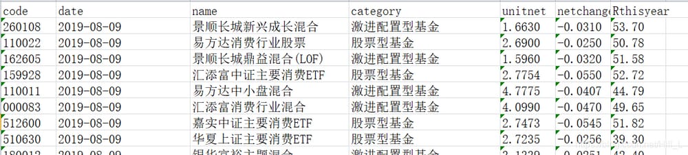
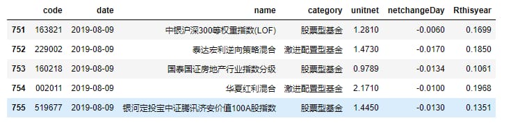
openF=pd.read_excel('D:/PythonData/OpenF.xlsx')
openF.head(3) #Check to see if there are any data exceptions.

このように表示されます。

# Rename the index to English name to facilitate data processing, see above that the 0 in front of the fund code is not recognized, read it to str format.
openF=pd.read_excel('D:/PythonData/OpenF.xlsx',converters = {u'fund code':str}) #
openF.rename(columns={'serial number':'NO.','fund code':'code','fund short name':'name','date':'date','unit net value':'unitnet','cumulative net value':'sumnet','dailygrowth':'Dailygrowth','last1 week':'Rweek','Last 1 month':'R1month','Last 3 months':'R3months','Last 6 months':'R6months','Last 1 year':'R1year','Last 2 years':'R2years','Last 3 years':'R3years','Since this year':'thisyear','SinceFoundation' :'SinceFounded','fees':'charges'},inplace=True)
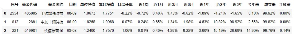
openF.head(3)

以下のように表示されます。

#Delete duplicate data sequences collected
openF.drop_duplicates(inplace=True)
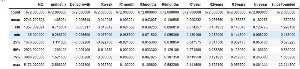
openF.describe()

# We want to be steady, 8 months so far this year, the SSE index is almost back to the original point, we want the fund to have a positive return this year.
type(openF.Dailygrowth[0]) #see its all str type, need to convert to integer type
#open_F=openF[{'Dailygrowth','Rweek'}].str.strip('%').astype(float)/100 not hashable, something is wrong, have to come one by one
temp=openF.replace('---',np.nan)
openF=temp.replace('--',np.nan)
openF.tail(100)
openF.dropna(replace=True) #find those funds that are more than 3 years old, delete the last three years return of Nan
#openF.count()

パーセンテージは文字列形式でインポートされているので、floatモードに変換する必要があります。

Dailygrowth=openF['Dailygrowth'].str.strip('%').astype(float)/100 
Rweek=openF['Rweek'].str.strip('%').astype(float)/100 
R1months=openF['R1month'].str.strip('%').astype(float)/100 
R3months=openF['R3months'].str.strip('%').astype(float)/100 
R6months=openF['R6months'].str.strip('%').astype(float)/100 
R1year=openF['R1year'].str.strip('%').astype(float)/100 
R2syears=openF['R2years'].str.strip('%').astype(float)/100
R3years=openF['R3years'].str.strip('%').astype(float)/100
thisyear=openF['thisyear'].str.strip('%').astype(float)/100
SinceFounded=openF['SinceFounded'].str.strip('%').astype(float)/100
charges=openF['Charges'].str.strip('%').astype(float)/100 

openF['Dailygrowth']=Dailygrowth
openF['Rweek']=Rweek
openF['R1month']=R1month
openF['R3months']=R3months
openF['R6months']=R6months
openF['R1year']=R1year
openF['R2years']=R2syears
openF['R3years']=R3years
openF['thisyear']=thisyear
openF['SinceFounded']=SinceFounded
openF['charges']=charges

データの可視化により、ファンドの全体状況をより直感的に把握することができます。可視化によって、データをより直感的に理解・把握し、データのパターンを発見し、可能性のあるいくつかの傾向について洞察することができます。
バーで表示するようにしました。

#openF.head(5)
#data visualization to have a visualization of the data
openF_charges=openF.groupby('charges').count()
openF_charges=openF_charges.reset_index()
openF_charges.head(2)

attr = ["{}".format(i*100)+str('%') for i in openF_charges['charges']]
#attr = [i for i in openF_charges['charges']]
v1 = [i for i in openF_charges['code']]
bar = Bar("Open Fund Charges Distribution Chart: ")
bar.add("number of funds", attr, v1, xaxis_interval=0, xaxis_rotate=80, yaxis_rotate=50)
bar

結果は次のようになります。

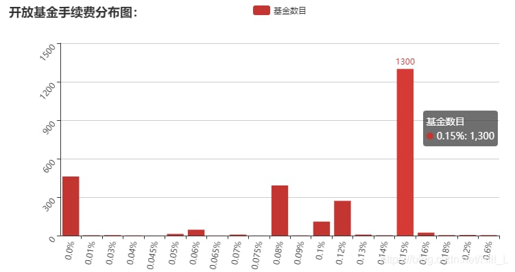
大半のファンドの手数料は0.15％で、1300円に達しています。これは現時点では比較的普通の手数料で、アリペイのファンド手数料のほとんどはこの範囲に収まっている。

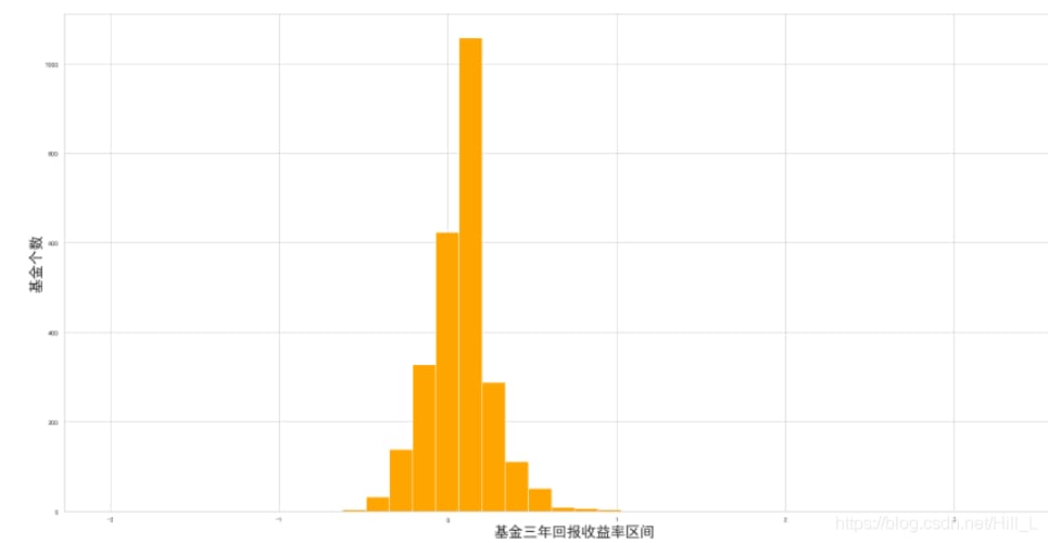
3年間のリターンが-20%から40%というのが、ほとんどのファンドの最終的なリターンです。

plt.rcParams['font.sans-serif']=['SimHei'] # to display Chinese labels normally
plt.rcParams['axes.unicode_minus']=False # to display the negative sign normally

from matplotlib.pyplot import MultipleLocator #coordinate interval change module
#ax=plt.gca() #reset the X coordinate interval
x_major_locator=MultipleLocator(0.5) #interval set to 0.5
ax.xaxis.set_major_locator(x_major_locator)

plt.xlabel(u'fund three-year return interval',fontsize=24)
plt.ylabel(u'number of funds',fontsize=24)
plt.hist(openF.R3years,bins=40,range=(-2,3.5),color='orange')

<イグ
同様に、今年のファンドのリターンを分析すると、同様の成果を上げている。

plt.rcParams['font.sans-serif']=['SimHei'] # used to display Chinese labels normally
plt.rcParams['axes.unicode_minus']=False #used to display the negative sign normally
# with Chinese appearances, need u'content'

ax=plt.gca() #reset the X coordinate interval
x_major_locator=MultipleLocator(0.1) #interval set to 0.5
ax.xaxis.set_major_locator(x_major_locator)

plt.xlabel(u'this year's return',fontsize=24)
plt.ylabel(u'number of funds',fontsize=24)
plt.hist(openF.thisyear,bins=40,range=(-0.2,1),color='red')
openF.thisyear.describe()

<イグ
0％～25％のリターンは、今年8月までにほとんどのファンドが達成したもので、全体としては昨年2018年よりかなり良くなっています。

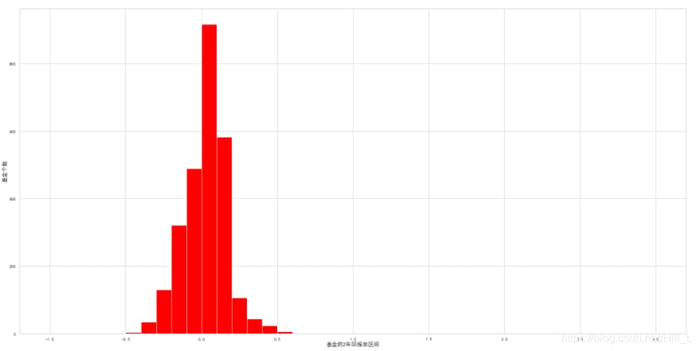
#Analysis of two-year returns
plt.rcParams['font.sans-serif']=['SimHei'] #used to display Chinese labels properly
plt.rcParams['axes.unicode_minus']=False # to display the negative sign normally

ax=plt.gca() #reset the X coordinate interval
x_major_locator=MultipleLocator(0.5) #set interval to 0.5
ax.xaxis.set_major_locator(x_major_locator)

plt.xlabel(u'fund's 2-year return interval',fontsize=14)
plt.ylabel(u'number of funds',fontsize=14)
plt.hist(openF.R2years,bins=40,range=(-1,3),color='red')
openF.R2years.describe()

2年間のファンドリターンは以下の通りです。-40％～20％が大半を占め、2年間のファンドリターンを最も集計したものが

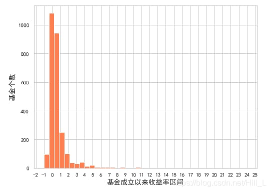
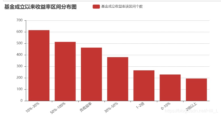
以下は、設立以来リターンが各レンジにあったファンド数の統計の続きである。設立以来リターンが2倍になったファンドは極めて少なく、20倍以上に達したファンドは非常に稀である。

その直後に、異なる満期、異なる間隔の基準収益率を少し分析することで、投資収益目標を合理的に設定することができるようになります。

""""The intention here is to use mapping for yield range classification, which fails!
R3years_to_Rank={
                      openF.R3years<0:"Bad",
(0<openF.R3years) & (openF.R3years<0.1): "0-10%",
(0.1<openF.R3years) & (openF.R3years<0.3):"10%-30%",
(0.3<openF.R3years) & (openF.R3years<0.5):"30%-50%",
                        openF.R3years>0.5:">50%"}
#'Series' objects are mutable, thus they cannot be hashed
openF['Rank']=openF.map(R3years_to_Rank)
openF.head() 
"""
#We prefer to see a more specific picture of the returns, which can be achieved by bar, a discretization of the continuous data.
# Call the cut function to process the data. pd.cut is used for faceting or discretization. cats=pd.cut(list,bins) bins is the interval passed in, available right=False for right open intervals. The return value cats has both .levels and label.
#3.0 has been changed to cats.codes and cats.categories.
bins=[openF.R3years.min(),0,0.1,0.3,0.5,1,2,openF.R3years.max()]
group_names=['negative_yield','0-10%','10%-30%','30%-50%','50%-100%','1-2x','2x+']
cats=pd.cut(openF.R3years,bins,labels=group_names,right=False)
#print(cats.codes) # can't call, maybe the new version has changed again
#print(cats.categories)
s1=pd.value_counts(cats)
attr=s1.index
v1=s1.values
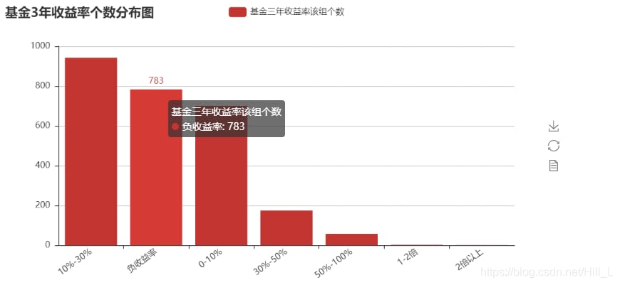
bar = Bar("Fund 3-year return number distribution")
bar.add("Fund 3 year returns for this group", attr,v1, xaxis_interval=0, xaxis_rotate=36, yaxis_rotate=0) Insert code snippet here

結果は次のようになります。

リターンがマイナスのファンドが783本あります。このように、ファンドへの投資はリスクが小さくないことがわかります。同時に、10％～30％、加えて0～10％のファンドも過半数を占めている。このように、超過リターンを狙うなら、30％以上のファンドを選ぶこと、これはかなり難しい作業である。
この2年間のファンド市場、分析に入りましょう。

# Do the same for 2-year returns
bins=[openF.R2years.min(),0,0.1,0.3,0.5,1,2,openF.R2years.max()]
group_names=['negative_yield','0-10%','10%-30%','30%-50%','50%-100%','1-2x','2x+']
cats=pd.cut(openF.R2years,bins,labels=group_names,right=False)
#print(cats.codes) # can't call, maybe the new version has changed again
#print(cats.categories)
s1=pd.value_counts(cats)
attr=s1.index
v1=s1.values


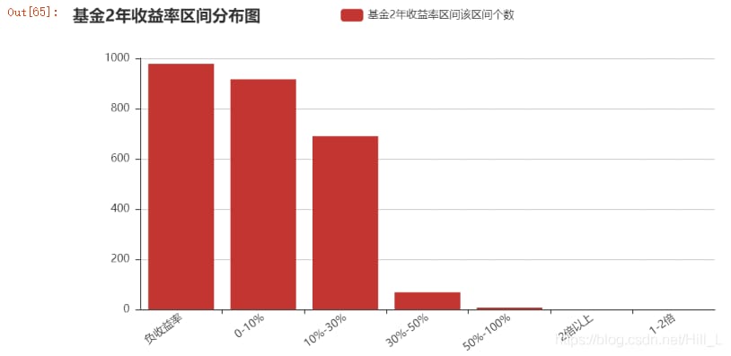
bar = Bar("Fund 2-year return interval distribution")
bar.add("Fund 2-year return interval the number of intervals", attr,v1, xaxis_interval=0, xaxis_rotate=36, yaxis_rotate=0)

<イグ
マイナスリターンが1番で、2番目が0～10％のリターンです。投資のベースがない人は、本当は銀行にお金を預けた方がいいんです。30％以上のリターンのファンドは努力すべき目標だが、かなりの努力が必要だ。

次に、ファンドの設定時からのリターンを分析します。分析するのに適した次元は、実は年率換算したリターンですが、ここでは紹介しません。これは、ファンドの設立と連動した二次的な分析が必要であり、興味のある読者は試してみるとよいだろう。

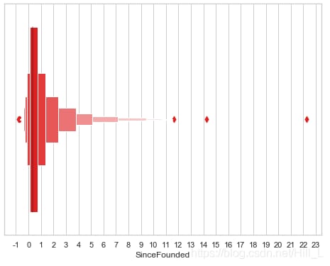
#For the level of concentration, you can use the box plot to see
sns.set(style="whitegrid")
ax=plt.gca() #reset x-coordinate interval
x_major_locator=MultipleLocator(1) # interval set to 1

ax.xaxis.set_major_locator(x_major_locator)
ax = sns.boxenplot(x=openF['SinceFounded'],color='red')

<イグ
11倍を超えるポイントが3つあります。データ分析レポートをするときに、これらの資金に着目して分析を取り出すことができます。

最初のグランドファンドスクリーニングを開始するために。

# selected a fee of less than 0.15%. This will ensure the fund's stability, ability to grow, and ability to withstand risk.
#We want to be robust, so far this year, 8 months, the Sensex is almost back to the original point, we want the fund to have a positive return this year.
temp=openF[(openF.charges<0.0015)&(openF.R3years>0)&(openF.thisyear>0)&(openF.R1year>0)&(openF. SinceFounded>0)]
temp.head()
openF_total=temp #openF at this time to retain those funds that initially have investment value

ここでとりあえず第一段階は終了し、歩留まりを中心とした分析に入ります。

次に、ステップ2です。この第2ステップでは、ファンドの種類別分布とモーニングスターの格付けに注目します。モーニングスターの格付けについては、三つ星以上のファンドを選んで注目した。

# In addition, crawled open-end funds with a Morningstar rating of 3 and 5 years with an investment return rating of 3 stars or more, with attributes such as fund type, % return this year, and fund net worth.
df_R=pd.read_excel('D:/PythonData/RankOpenF.xlsx',converters = {u'code':str})
df_R['Rthisyear']=df_R.Rthisyear/100
# df_R=df_R.set_index('code')
df_R.tail(5) # see if the data is normal

データはOKです。

ファンド全体を、レーティング、タイプを組み合わせて視覚的に分析したもの。

df_R_category=df_R.category.value_counts()
df_R_category.index

attr = df_R_category.index
v1 = df_R_category.values
bar = Bar("Distribution of fund types with all Morningstar ratings over 3 stars")
bar.add("Number of funds with a Morningstar rating of 3 stars or more", attr, v1, xaxis_interval=0, xaxis_rotate=36, yaxis_rotate=0)
bar

その結果は以下のとおりです。アグレッシブアロケーションファンドや株式・アグレッシブボンドファンドなど、比較的良質なファンドが多い。また、ベースが比較的大きいことも関係している可能性があり、ここでは比例分析との組み合わせが良いと思われます。

条件を組み合わせて、以下のようにフィルタリングします。

# After the initial screening of fund data, further screening is performed in combination with Morningstar ratings. Funds can be further narrowed down.
print(df_R[df_R.code=='110003'])
print(openF[openF.code=='110003'])
df_RF=pd.merge(openF,df_R,on='code') #,suffixes=('_df_R','_openF')
df_RF_copy=df_RF.copy() # make a copy of the data spare
df_RF.head(1)
df_RF=df_RF.drop(columns=['date_y','name_y','unitnet_y','Rthisyear']) # remove duplicate columns of attributes
df_RF_CX=df_RF
df_RF_CX.describe()

設立以来、平均リターンは1.57と堅調に推移しています。Morningstar.comの3つ星以上のファンドに今年投資した場合の期待リターンは18.2%で、全体としてはまだ良い方である。最大は2.2倍になり、最小は18％の損失である。その差は決して小さくはない。

上記はMorningstar.comと連動したデータ分析で、その直後に配当を見ています。

第3段階は配当の検討ですが、一般的には配当をより考慮した銘柄を選びます。このあたりはファンドはあまり応用がきかないので、少し検証してみましょう。ただ、総合的には、配当のないファンドより配当のあるファンドの方が良いと思います。

divF=pd.read_excel('D:/PythonData/divF.xlsx',converters = {'code':str})
print(divF.head(1))
#print(divF.describe())

#import a fund's dividend data, including the number of dividends and the amount of dividends per share
from datetime import datetime
%matplotlib inline
plt.rcParams['figure.figuresize'] = (30.0, 15.0)


divF = pd.read_excel('D:/PythonData/divF.xlsx',converters = {'code':str})
#print(divF.head(3))

データは以下のように表示されます。

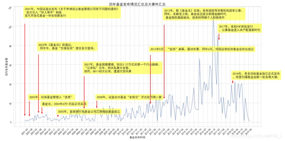
ファンドの発行本数との関係で、その歴史を簡単に見てみると面白い。

divF['FoundDate2']=pd.to_datetime(divF['FoundDate'])
df=divF[['FoundDate2','code']]
df['Month'] = [datetime.strftime(x,'%Y-%m') for x in df['FoundDate2']]
df =df.pivot_table(index='Month',aggfunc='count')

fig=plt.figure()
ax=fig.add_subplot(111)

x_major_locator=MultipleLocator(4)
ax.xaxis.set_major_locator(x_major_locator)# set the main scale of the x-axis to a multiple of 3

plt.title('Summary of fund releases and summary of major events over the years',fontsize=24) # set the chart title and title font size
plt.tick_params(axis='both',which='major',labelsize=16,rotation=45) #set the font size of the scale
plt.xlabel('fund release time',fontsize=18)#set the x-axis label and its font size
plt.ylabel('Number of funds released in the month',fontsize=18)#set the x-axis label and its font size


#Funds big thing.

plt.annotate(u'In 2001, the CSRC issued the "Notice on Certain Issues Concerning the Application for the Establishment of Fund Management Companies"\n the first introduction of the "good guys raising their hands" system\n the first open-end fund-Hua'an Innovation Issue',
   xy=('2001-04',1),xytext=('2001-04',110), 
   bbox = dict(boxstyle = 'round,pad=0.5',
   fc = 'yellow', alpha = 0.5),
   arrowprops = dict(facecolor='red', 
   shrink=0.05),fontsize=20)

plt.annotate(u'2002, Social Security Fund Manager "Selection"',
   xy=('2002-08',5),xytext=('2002-08',25), 
   bbox = dict(boxstyle = 'round,pad=0.5',
   fc = 'yellow', alpha = 0.5),
   arrowprops = dict(facecolor='red', 
   shrink=0.05),fontsize=20)

plt.annotate(u'2003 "Fund Law" was passed, \n the same year, the fund "value investment" concept debuted.' ,
   xy=('2003-08',6),xytext=('2003-08',76), 
   bbox = dict(boxstyle = 'round,pad=0.5',
   fc = 'yellow', alpha = 0.5),
   arrowprops = dict(facecolor='red', 
   shrink=0.05),fontsize=20)

plt.annotate(u'Fund Law, effective June 1, 2004',
   xy=('2003-12',8),xytext=('2003-12',18), 
   bbox = dict(boxstyle = 'round,pad=0.5',
   fc = 'yellow', alpha = 0.5),
   arrowprops = dict(facecolor='red', 
   shrink=0.05),fontsize=20)


plt.annotate(u'2005, the first bank-based fund company ICBC Credit Suisse Fund was established',
   xy=('2005-04',5),xytext=('2005-04',10), 
   bbox = dict(boxstyle = 'round,pad=0.5',
   fc = 'yellow', alpha = 0.5),
   arrowprops = dict(facecolor='red', 
   shrink=0.05),fontsize=20)

plt.annotate(u'In 2007, the fund size exploded, hitting the first industry peak of 3.27 trillion. \nThe first year of the "public run private", the sunshine private development. \nHowever, QDII first went to sea and encountered the subprime mortgage storm',
   xy=('2007-04',12),xytext=('2007-04',52), 
   bbox = dict(boxstyle = 'round,pad=0.5',
   fc = 'yellow', alpha = 0.5),
   arrowprops = dict(facecolor='red', 
   shrink=0.05),fontsize=20)


plt.annotate(u'2008, the Securities and Exchange Commission on the fund "mouse position" issued the first single punishment ',
   xy=('2008-04',14),xytext=('2008-04',25), 
   bbox = dict(boxstyle = 'round,pad=0.5',
   fc = 'yellow', alpha = 0.5),
   arrowprops = dict(facecolor='red', 
   shrink=0.05),fontsize=20)


plt.annotate(u'In May 2012, the curtain fell on "Hong Wei", shaking China. In June of the same year, the China Securities Investment Fund Association was established',
   xy=('2012-04',16),xytext=('2012-04',75), 
   bbox = dict(boxstyle = 'round,pad=0.5',
   fc = 'yellow', alpha = 0.5),
   arrowprops = dict(facecolor='red', 
   shrink=0.05),fontsize=20)


plt.annotate(u'2013, the implementation of the new Fund Law; brokerage firms insurance and other capital management institutions into the public offering. \nThe same year, the balance of the treasure online, the fund industry into the era of Internet finance,\n Fund equity incentives to break the ice, the State Council clarified the conditions of personal shareholding ',
   xy=('2013-04',20),xytext=('2013-04',108), 
   bbox = dict(boxstyle = 'round,pad=0.5',
   fc = 'yellow', alpha = 0.5),
   arrowprops = dict(facecolor='red', 
   shrink=0.05),fontsize=20)

plt.annotate(u'2017, the first batch of FOF approved for issue \n, public funds into a new era of asset allocation',
   xy=('2017-04',85),xytext=('2017-04',95), 
   bbox = dict(boxstyle = 'round,pad=0.5',
   fc = 'yellow', alpha = 0.5),
   arrowprops = dict(facecolor='red', 
   shrink=0.05),fontsize=20)

plt.annotate(u'2018, pension target fund guidelines officially released \n, is expected to trigger a new round of fund industry development tide.' ,
   xy=('2018-04',40),xytext=('2018-04',46), 
   bbox = dict(boxstyle = 'round,pad=0.5',
   fc = 'yellow', alpha = 0.5),
   arrowprops = dict(facecolor='red', 
   shrink=0.05),fontsize=20)


plt.plot(df.index,df.code)



plt.show()

結果は以下の通りです。楽しいでしょう？

ファンドの分配金についてご紹介します。

#coding:utf-8
import matplotlib.pyplot as plt
plt.rcParams['font.sans-serif']=['SimHei'] # to display Chinese labels normally
plt.rcParams['axes.unicode_minus']=False #used to display the negative sign normally
# with Chinese appearances, need u'content'

ax=plt.gca()
x_major_locator=MultipleLocator(10) #interval set to 10
ax.xaxis.set_major_locator(x_major_locator)

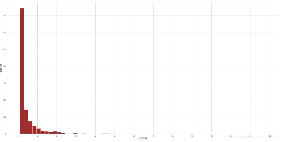
plt.xlabel(u'number of dividends',fontsize=14)
plt.ylabel(u'number of funds',fontsize=14)
plt.hist(divF.div_count,bins=60,color='brown')

ax=plt.gca()
x_major_locator=MultipleLocator(1) # interval set to 1
ax.xaxis.set_major_locator(x_major_locator)

plt.xlabel(u'total dividend amount',fontsize=14)
plt.ylabel(u'number of funds',fontsize=14)
plt.hist(divF.div_sum,bins=50,color='brown')

<イグ

配当回数と配当額ですが、配当の大半は1回のみで、配当額はすべて0.5ドル以内に収まっているものがほぼ占めています。
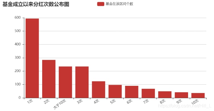
配当回数を間隔に分けると、次のような結果になります。

bins=[1,2,3,4,5,6,7,8,9,10,11,divF.div_count.max()]


group_names=['1 time','2 times','3 times','4 times','5 times','6 times','7 times','8 times','9 times','10 times','greater than 10 times']

cats=pd.cut(divF.div_count,bins,labels=group_names,right=True)

s1=pd.value_counts(cats)
attr=s1.index
v1=s1.values

bar = Bar("Fund inception since the number of dividends announced graph")
bar.add("Number of funds in the interval", attr,v1, xaxis_interval=0, xaxis_rotate=36, yaxis_rotate=0)

<イグ
配当金の額は以下のとおりです。

bins=[0,0.1,0.2,0.5,0.8,1,2,5,divF.div_sum.max()]
cats=pd.cut(divF.div_sum,bins,right=False)

s1=pd.value_counts(cats)
attr=s1.index
v1=s1.values

bar = Bar("fund since the inception of the dividend amount announced graph (unit: $) ")
bar.add("Number of funds in the interval", attr,v1, xaxis_interval=0, xaxis_rotate=36, yaxis_rotate=0)

ご覧の通り、ペニー配当の額は多いですね。
次に、このステップの結果としてのデータの予備的なフィルタリングを行い、それを保存します。以下のように。

divF.head(2)
print(divF.count())
#Dividends may be affected by the fund's time to market, but we still want the fund to pay out more than 2 dividends and the dividend amount to be located above the average value of $0.32. This will allow us to have a more robust investment strategy.
divF_total=divF[(divF.div_count>2) & (divF.div_sum>0.32)]
divF_last=divF_total
print(divF_last.describe())

第4ステップでは、証券会社の格付けとの関連でデータを分析する必要があります。格付け機関は、上海証券、中国招商証券、済南金信である。

#read_daily_funds.com rating data, if you need pivot data, excel pivot view is more efficient.
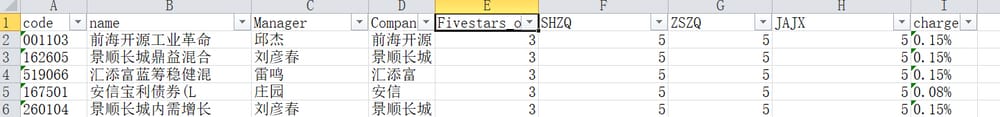
df_T=pd.read_excel('D:/PythonData/tiantianRank.xlsx',converters = {u'code':str})
df_T.tail(5) # data null exists

結果は次のようになります。

charge=df_T['charge'].str.strip('%').astype(float)/100
df_T['charge']=charge
#df_T.describe() #count reflects the number of null values and is consistent

#look at the distribution of five-star ratings given by each fund rating company
df_T.pivot_table(index=['Fivestars_of_count'],aggfunc='count')

# Look at the distribution across companies
df_T.pivot_table(index=['Fivestars_of_count'],columns=['Company'],aggfunc='count')

Distribution of ratings given to different fund companies by the #three rating companies
df_T.pivot_table(index=['Company'],columns=['Fivestars_of_count'],aggfunc='count')

# Distribution of ratings given by a particular rating company for each fund company
df_T.pivot_table(index=['SHZQ'],columns=['Company'],aggfunc='count',margins_name='Company')

# At the pivot level, excel can directly derive pivot charts based on pivot tables, so turn to excel for analysis of fund quality distribution, top fund companies and top fund managers, etc.

#The three rating agencies given in the daily fund include China Merchants Securities/Shanghai Securities/Jian Jinxin, what are their screening results, let's see. Its rating has been floating point, if you choose more than four stars is also convenient arithmetic.
# For now, we have no shortage of good funds, continue to screen with the strict conditions of 3 five-star ratings.
df_T.head(2)
df_T_total=df_T[df_T.Fivestars_of_count==3]
df_T_total.describe() # Look at 52 more. Not much.
df_T_last=df_T_total

# Finally, it is the investor is concerned about, under the support of big data, which funds are worth investing in.
#The DataFrame data openF_total, which is more about yield and stability of returns, is the initial screening of the funds we did earlier.
openF_total.describe()

構造的な整合性を確保するために、Excelのピボット・テーブルの一部を使ったピボット・チャートを示します。

# And then combined with Morningstar.com's three-star rating or higher, we do a secondary screening, also resulting in another DataFrame, df_RF_CX
df_RF_CX.describe() #We see that there are 295 more funds, which is still a bit much for selection. Continue the handsome selection using data from the three securities rating companies. Excellent funds after combining data from Morningstar.com.


#combined with calendar year dividend amounts and dividend data, we also get a DateFrame. divF_total
divF_last.describe() #A total of 544.

# Funds that received 5-star ratings from all three rating companies, as follows.
df_T_last.describe() # 52 in total

5番目の部分は、上記の結果を組み合わせたものに相当し、最終的なファイルとして、パソコンに保存することを選択しました。これでデータ解析のステップは終了です。

#Finally, it's time to see the birth of a quality base.
df1=pd.merge(df_RF_CX,divF_last,on='code') # Combined yield, Morningstar rating and dividends three factors.

df2=pd.merge(df1,df_T_last,on='code') # on top of df1, plus the ratings of the three major securities companies.

result=df2.T.drop_duplicates().T

WorthyOfInvestment=result.drop(columns=result['name_x']) # see some sites on the naming display abbreviations, we take a column can be.

WorthyOfInvestment.to_excel('D:/PythonData/QualityInvestmentFundsAugust2019.xlsx')

ファンドの推奨を疑われないよう、その最終結果は以下のように一部傍証しています：ICBC金融不動産以外のファンドはすべて古いものです。彼らは時の試練に耐えており、今後も私たちを驚かせてくれると信じています。設立以来の古いファンドが2本あり、さらに10倍の収益率です。そして、2013年の比較的新しいものも、利回り2.4倍です。年率15％の複利利回りはとても頼もしいです。(長年にわたる金融不動産セクターの株式の引き上げのおかげです）。

第五部 洞察と結論

ここでは、分析の主なプロセスステップを、技術的な実装とともに説明する。主な分析部分はデータ分析レポートに配置し、ここでは分析の簡単な結論を述べています。
1) 今年のファンド投資の収益率は、昨年のファンド投資の収益率よりはるかに良い、昨年はファンドをやって、おそらくローは損失状況に直面した。
2）15％の期待収益率は、比較的到達するのは難しいしきい値ですが、約10％、現在のファンドの収益率によると、確率は達成可能です。
3）エファタル、景春長城、銭海開源という3社のファンドは全体的に品質がよく、評価については、私たちが選んだデータのリターンと合わせて、少なくとも5つ星評価のファンドは私たちの長期投資にとって非常に重要な参考対象である。
4）良いファンドマネージャーを選択し、彼のファンドを追跡することは本当に私たちがより多くの心の平和と投資することができ、良いファンドマネージャー、非常に重要である。
5) 投資のアドバイスを一文でまとめると、良いファンド、良いファンド会社、良いファンドマネージャー、良いタイミング、良い期待値、良い利回りということになります。