Python_matplotlib の凡例は外側に保存すると不完全になる

前回も触れましたが、以下のコードでベクトルプロットを保存すると、外側に配置された凡例が不完全に表示されることがよくあります。

import numpy as np
import matplotlib.pyplot as plt
fig, ax = plt.subplots()
x1 = np.random.uniform(-10, 10, size=20)
x2 = np.random.uniform(-10, 10, size=20)
#print(x1)
#print(x2)
number = []
x11 = []
x12 = []
for i in range(20):
    number.append(i+1)
    x11.append(i+1)
    x12.append(i+1)
plt.figure(1)
# you can specify the marker size two ways directly:
plt.plot(number, x1, 'bo', markersize=20,label='a') # blue circle with size 20
plt.plot(number, x2, 'ro', ms=10,label='b') # ms is just an alias for markersize

lgnd=plt.legend(bbox_to_anchor=(1.05, 1), loc=2, borderaxespad=0,numpoints=1,fontsize=10)
lgnd.legendHandles[0]. _legmarker.set_markersize(16)
lgnd.legendHandles[1]. _legmarker.set_markersize(10)

plt.show()

fig.savefig('scatter.png',dpi=600)

scatter.pngとして保存した後の効果は以下の通りです。

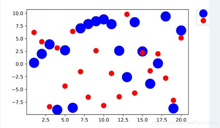
画像の右上に配置された凡例は、左側のほんの一部しか表示されていないことがわかります。

その理由は簡単で、savefig()関数を使ってベクター画像を保存するとき、その画像はバウンディングボックス（bbox）で囲まれ、その中に入る画像だけが保存されるので、凡例がそのボックス内に完全に入らない場合、保存されないからです。

仕組みが分かれば、問題解決も簡単です。

ここで、2つの解決策を提案します。

1. bboxに完全に入らない画像を取り、完全に入るように移動させれば、bboxに遮られた画像が完成する（画像をbboxの中に移動させる）。

2. 特にbboxの外に落ちやすい凡例については、その画像を完全に含むようにbboxのサイズを変更する（bboxを拡張して画像を完全に含むようにする）。

この問題を解決するために、それぞれの考え方に基づく2つのアプローチを以下に紹介します。

1. 関数を使用する subplots_adjust()

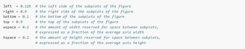
公式ドキュメントにあるように、subplots_adjust()関数はサブプロットのレイアウトを調整するために使用されます。6つのパラメータを持ち、そのうち4つはleft, right, bottom, topでそれぞれサブプロットの左、右、下、上の位置を調整し、残りの2つのパラメータwspace, hspaceでサブグラフ間の左右および上下の距離を調整する。

初期値は以下の通りです。

上の図を例にして、今度は凡例から考えてみましょう。 右側 が表示されていない場合、subplots_adjust()関数のrightパラメータを調整して、その位置を少し左にずらし、rightパラメータのデフォルト値を0.9から0.8に変更すると、次のように完全な凡例が得られます。

import numpy as np
import matplotlib.pyplot as plt
fig, ax = plt.subplots()
x1 = np.random.uniform(-10, 10, size=20)
x2 = np.random.uniform(-10, 10, size=20)
#print(x1)
#print(x2)
number = []
x11 = []
x12 = []
for i in range(20):
    number.append(i+1)
    x11.append(i+1)
    x12.append(i+1)
plt.figure(1)
# you can specify the marker size two ways directly:
plt.plot(number, x1, 'bo', markersize=20,label='a') # blue circle with size 20
plt.plot(number, x2, 'ro', ms=10,label='b') # ms is just an alias for markersize

lgnd=plt.legend(bbox_to_anchor=(1.05, 1), loc=2, borderaxespad=0,numpoints=1,fontsize=10)
lgnd.legendHandles[0]. _legmarker.set_markersize(16)
lgnd.legendHandles[1]. _legmarker.set_markersize(10)

fig.subplots_adjust(right=0.8)

plt.show()

fig.savefig('scatter1.png',dpi=600)

scatter1.png として保存した後、scatter.png との比較は次のようになります。

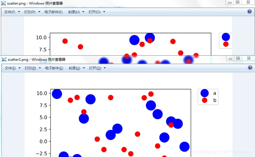
scatter1.pngの凡例が全体的に表示されていることがわかります。これは、画像の右側の位置を左にずらして、全体として保存された画像に含まれることで行われます。

同様に、凡例が画像の下側にある場合、savefig() で保存すると不完全になるので、関数 subplots_adjust() を修正して、保存のために画像を横取りするボックス、すなわち後述の bbox に含まれるように上に移動する必要があります。

import numpy as np
import matplotlib.pyplot as plt
fig, ax = plt.subplots()
x1 = np.random.uniform(-10, 10, size=20)
x2 = np.random.uniform(-10, 10, size=20)
#print(x1)
#print(x2)
number = []
x11 = []
x12 = []
for i in range(20):
    number.append(i+1)
    x11.append(i+1)
    x12.append(i+1)
plt.figure(1)
# you can specify the marker size two ways directly:
plt.plot(number, x1, 'bo', markersize=20,label='a') # blue circle with size 20
plt.plot(number, x2, 'ro', ms=10,label='b') # ms is just an alias for markersize

lgnd=plt.legend(bbox_to_anchor=(0.4, -0.1), loc=2, borderaxespad=0,numpoints=1,fontsize=10)
lgnd.legendHandles[0]. _legmarker.set_markersize(16)
lgnd.legendHandles[1]. _legmarker.set_markersize(10)

plt.show()
fig.savefig('scatter#1.png',dpi=600)

というのは subplots_adjust() はデフォルトの底値が0.1なので、底を上に移動するために fig.subplots_adjust(bottom=0.2) を追加し、次のように修正します。 

import numpy as np
import matplotlib.pyplot as plt
fig, ax = plt.subplots()
x1 = np.random.uniform(-10, 10, size=20)
x2 = np.random.uniform(-10, 10, size=20)
#print(x1)
#print(x2)
number = []
x11 = []
x12 = []
for i in range(20):
    number.append(i+1)
    x11.append(i+1)
    x12.append(i+1)
plt.figure(1)
# you can specify the marker size two ways directly:
plt.plot(number, x1, 'bo', markersize=20,label='a') # blue circle with size 20
plt.plot(number, x2, 'ro', ms=10,label='b') # ms is just an alias for markersize

lgnd=plt.legend(bbox_to_anchor=(0.4, -0.1), loc=2, borderaxespad=0,numpoints=1,fontsize=10)
lgnd.legendHandles[0]. _legmarker.set_markersize(16)
lgnd.legendHandles[1]. _legmarker.set_markersize(10)

fig.subplots_adjust(bottom=0.2)

plt.show()
fig.savefig('scatter#1.png',dpi=600)

効果の比較

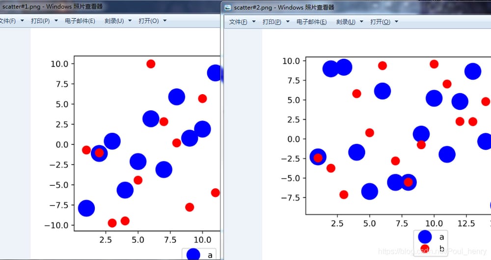
他の場所でも凡例は同じです。 

2. 関数を使用する savefig()

前回のブログで紹介したように、savefig()関数のfname、dpi、formatの3つの引数でベクター画像を保存することができますが、今度は関数のもう一つの引数である bbox_inches を作る

グラフに保存されていない凡例を含める。

下図に示すように、bbox_inchesはグラフのbbox、すなわちバウンディングボックスを調整する役割を果たします。

 ご覧のように、bbox_inchesを「tight」に設定すると、その画像からよりタイトな（きつい）バウンディングボックスのbboxを計算し、その選択したボックスで画像を保存することができます。

ここでいうタイトなバウンディングボックスは、画像を完全に含む矩形であるべきですが、画像から一定のパディング距離を置いて、同じように 最小バウンディングボックス (ミニマムバウンディングボックス)ですが、個人的には、若干の違いがあります。単位もインチです。

こうすることで、凡例がbboxに含まれるようになり、その結果、保存されます。

フルコードです。

import numpy as np
import matplotlib.pyplot as plt
fig, ax = plt.subplots()
x1 = np.random.uniform(-10, 10, size=20)
x2 = np.random.uniform(-10, 10, size=20)
#print(x1)
#print(x2)
number = []
x11 = []
x12 = []
for i in range(20):
    number.append(i+1)
    x11.append(i+1)
    x12.append(i+1)
plt.figure(1)
# you can specify the marker size two ways directly:
plt.plot(number, x1, 'bo', markersize=20,label='a') # blue circle with size 20
plt.plot(number, x2, 'ro', ms=10,label='b') # ms is just an alias for markersize

lgnd=plt.legend(bbox_to_anchor=(1.05, 1), loc=2, borderaxespad=0,numpoints=1,fontsize=10)
lgnd.legendHandles[0]. _legmarker.set_markersize(16)
lgnd.legendHandles[1]. _legmarker.set_markersize(10)

#fig.subplots_adjust(right=0.8)

plt.show()

fig.savefig('scatter2.png',dpi=600,bbox_inches='height')

scatter2.pngとして保存された、scatter.png、scatter1.png、scatter2.pngの比較画像です。

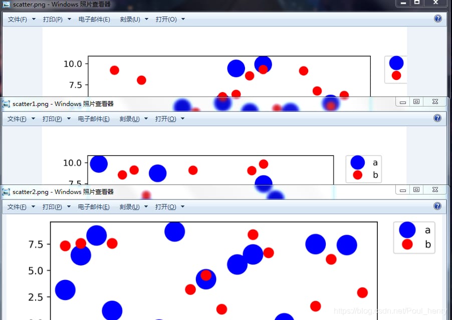
ご覧のように、最初の方法であるscatter1.pngの考え方は、切片を保存するために使用したbboxをそのままにして、画像の右端を左に移動させることであり、2番目の方法であるscatter2.pngの考え方は、切片を保存するために使用したbboxをそのまま画像全体に拡大しながら、すべてを含めることである。

備考 : savefig() には、さらに2つの指定パラメータがあります。

そのうちの1つは パッドインチス これは、直前の bbox_inches が 'tight' である場合に、画像と bbox の間のパディングの距離を調整するために使用されますが、ここでは設定する必要がなく、デフォルト値を選択するだけです。

個人的には、pad_inches パラメータを 0、つまり pad_inches=0 にすると、切片が保存される bbox は最小バウンディングボックスとなります。 

もうひとつは bbox_extra_artists これは、画像のbboxを計算して他の要素も含めるために使用されます。

例として、画像の左側に別のテキストボックスのテキストを追加し、画像保存時にそのテキストボックスをbboxに含めたい場合、パラメータbbox_extra_artistsを使ってテキストを含めることができます（実際には、bbox_extra_artistsが使われていなくても保存画像にテキストは含まれます）。

import numpy as np
import matplotlib.pyplot as plt
fig, ax = plt.subplots()
x1 = np.random.uniform(-10, 10, size=20)
x2 = np.random.uniform(-10, 10, size=20)
#print(x1)
#print(x2)
number = []
x11 = []
x12 = []
for i in range(20):
    number.append(i+1)
    x11.append(i+1)
    x12.append(i+1)
plt.figure(1)
# you can specify the marker size two ways directly:
plt.plot(number, x1, 'bo', markersize=20,label='a') # blue circle with size 20
plt.plot(number, x2, 'ro', ms=10,label='b') # ms is just an alias for markersize

lgnd=plt.legend(bbox_to_anchor=(1.05, 1), loc=2, borderaxespad=0,numpoints=1,fontsize=10)
lgnd.legendHandles[0]. _legmarker.set_markersize(16)
lgnd.legendHandles[1]. _legmarker.set_markersize(10)

text = ax.text(-0.3,1, "test", transform=ax.transAxes)

#fig.subplots_adjust(right=0.8)
plt.show()
fig.savefig('scatter3.png',dpi=600, bbox_extra_artists=(lgnd,text),bbox_inches='tight')

効果を表示します。

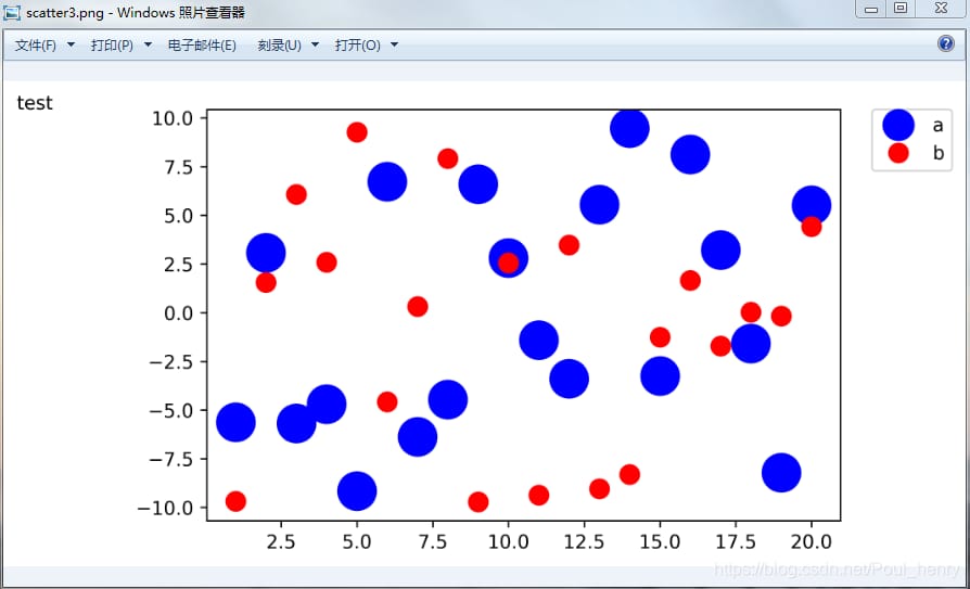
 bboxに含まれない要素がある場合、このパラメータを使用することを検討してください。